AI Inference: What happens after the model is trained?

Inspiration

This write-up is inspired by having to optimise Qwen3.5 for the AI-HPC26 competition. To know where to start optimising, you have to understand what happens inside LLMs.

Overview

Here is the general story. There are two parts to inference:

1. Prefill: the processing of the input tokens.
2. Decoding: the process of generating the output tokens.

When I say “during training,” for now, you can assume that to be true, at least until I write my next blog on AI pretraining/training.

Tokenizers

Let’s start with the famous example: The cat sat on the.

Depending on the tokenizer, this sentence can be broken up differently. In other words, the split varies across different tokenizers.

Tokenize by phrases: {"The cat", "sat", "on the"}
Tokenize by word:    {"The", "cat", "sat", "on", "the"}
Tokenize by parts:   {"Th", "e", "sat", "on", "th", "e"}

Think about it like this: there are different ways to predict or learn language, maybe by phrases, words, or parts. Modern LLMs usually use subword tokenization, where tokens can be whole words, word pieces, punctuation, spaces, or byte-level chunks depending on the tokenizer.

There are other tricks for breaking down special characters like emojis, symbols, and different languages into tokens. For example, maybe an emoji will be stored through its Unicode/byte representation instead of as the actual emoji you see on screen.

Mapping -> Embedding / Hidden State

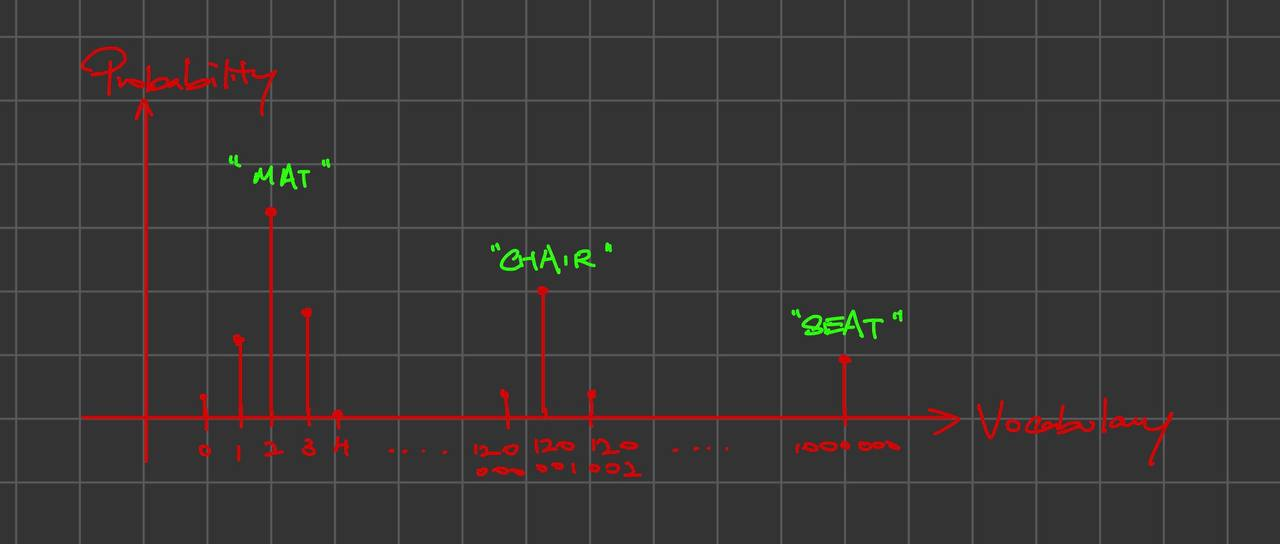
During training, the model has access to something called a vocabulary. Let’s just say it has a size of 1,000,000.

The tokenized parts get converted into numbers called token IDs. Most of the time, tokenizers are case-sensitive.

{"Th", "e", "sat", "on", "th", "e"}
-> {68, 4, 199764, 170, 10068, 4}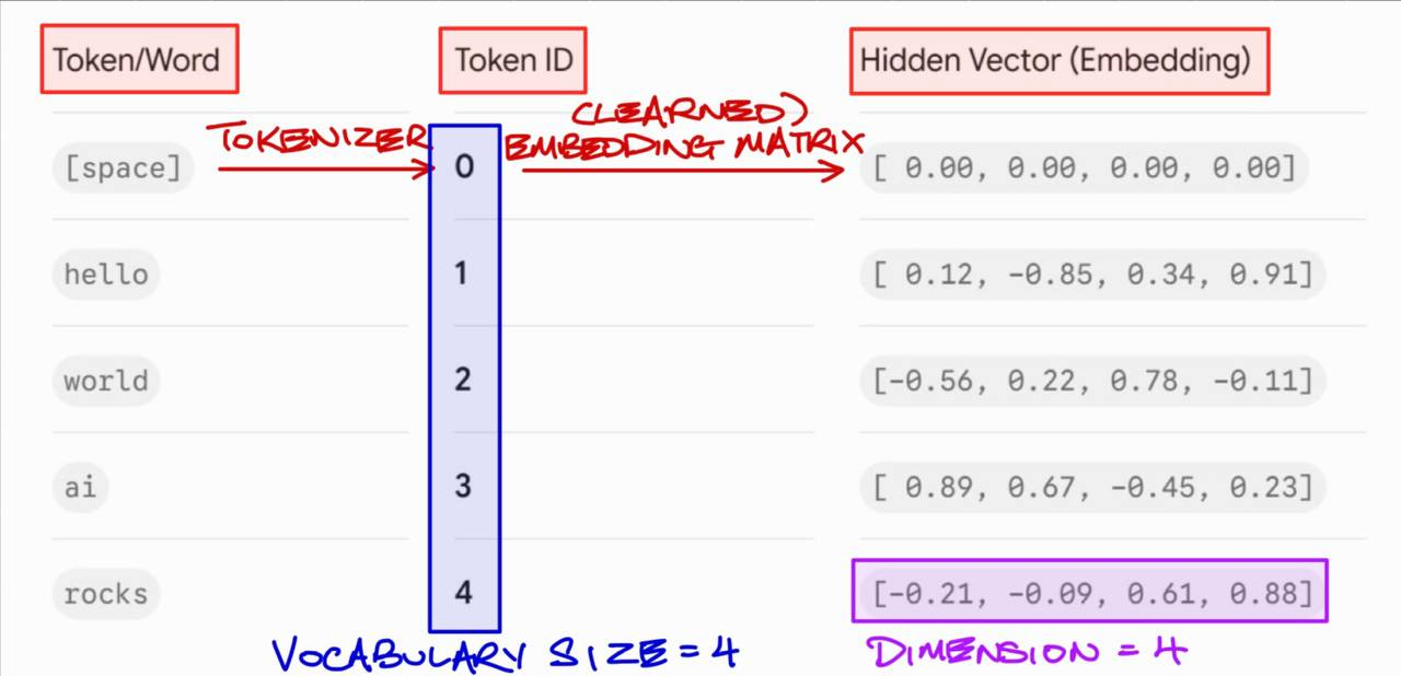

Each token ID indexes into an embedding table, producing a hidden vector of dimension d_model. Depending on the model, this might be hundreds, thousands, or more dimensions. For example, many large transformer models use hidden sizes such as 4096, but the exact number is architecture-specific.

Embedding Handling: RoPE -> KV Cache

More on this later.

During training, each attention head has learned projection matrices. You can think of them as dedicated matrices used to convert the embedding vector into three other vectors called Query (Q), Key (K), and Value (V). Usually, these matrices have a scaling effect on the embedding vector.

So, each attention layer has learned projection matrices that produce Q, K, and V vectors. Conceptually, each attention head gets its own Q/K/V projections, though implementations often store all heads together in large combined matrices for efficiency.

"cat sat on"

Q_cat, Q_sat, Q_on
K_cat, K_sat, K_on
V_cat, V_sat, V_on

Another key idea to take note of before continuing is the intuitive grasp of Rotary Positional Embedding (RoPE). In other words, this is how the model identifies the position of words.

For example, cat bit dog and dog bit cat have two different meanings based on where the words lie before and after bit.

RoPE is usually applied to the Query and Key vectors before the attention dot product. This injects positional information into the attention scores. The Value vectors are usually not RoPE-rotated.

Attention Score = RoPE(Q_cat, P1) dot RoPE(K_bit, P2)

Here, dot means dot product, and P1 is the position of cat in the initial prompt. Later, I’ll just use Q and K without writing RoPE every time, but mentally note that it is there.

Attention -> Multi-Head Attention (MHA)

Now that we know how embeddings are handled, we can define attention, which is the key trait that the learned projection matrices prioritise. Some heads may be good at paying attention to grammar, others to position, etc.

For context, let’s use this input:

The cat that I saw yesterday was sleeping

The high-level idea is:

1. Attention Score (A) = Q dot K
2. Softmax normalisation makes the terms sum to 1.
3. New Token Vector = A dot V

The actual formula is:

Attention(Q, K, V) = softmax((QK^T / sqrt(d_head)) + mask) V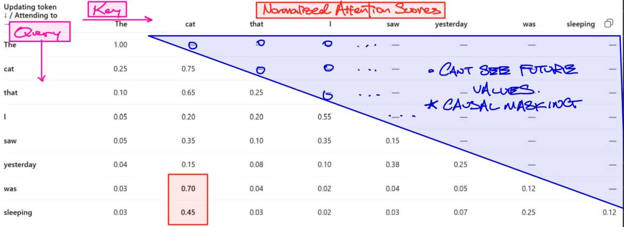

The model computes dot products between Queries and Keys, scales them, applies the causal mask, then uses softmax to turn them into attention weights. These weights are used to take a weighted sum of the Value vectors.

To reinforce the concepts, the current token is passed into multiple attention heads. An attention layer usually consists of 8, 16, 32, or 64 attention heads. These heads run in parallel and finish at the same time.

After all the heads are done processing, the model combines the results through concatenation. Finally, the output vector undergoes a linear projection, which mixes the result and converts the matrix back to the same number of dimensions as the original embedding vector.

Feed-Forward Network (FFN) / Multi-Layer Perceptron (MLP)

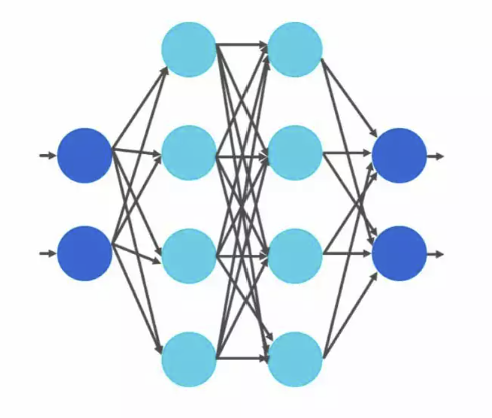
This layer is relatively straightforward:

1. The output vector from attention is scaled up, often around 4x.
2. A non-linear function is applied to its expanded form.
3. A linear projection matrix scales it back down to the original number of dimensions.

The FFN/MLP usually expands the hidden dimension, applies a non-linear activation such as GELU or SwiGLU, then projects it back down to the original hidden size. The expansion ratio is often around 4x, but modern models may use different ratios and gated activations.

Residual Stream

This is also relatively straightforward. If x is the original embedding vector we started from:

x1 = x + Attention(norm(x))
x2 = x1 + FFN(norm(x1))

Usually, a normalisation step, such as RMSNorm, happens around each subblock layer, like MHA or FFN, and then the result is added back into the next subblock stream.

A transformer layer usually consists of this MHA layer and FFN layer. Assuming there is only one transformer layer, we can now figure out how to handle the output and generate the next token. In practice, there are usually many more layers.

Generating the Next Token

Remember how we projected the initial token ID into an embedding. There is also another matrix that “unembeds” it. This is performed on x_output.

The unembedded output is known as logits. Subsequently, we apply softmax on the logits to get a distribution of probabilities for what word, or token, could come next.

Extra Settings

Remember, LLMs are still a probabilistic venture. The same prompt can produce varied outcomes:

"The cat sat on the"

Mat:   60 tickets
Floor: 20 tickets
Chair: 10 tickets
Bed:   10 tickets

Imagine a raffle. There is a chance for Floor to win, as well as a chance for Mat, Chair, and Bed.

There are other settings like temperature, which makes the distribution sharper or flatter. A lower temperature might look like this instead:

Mat:   80 tickets
Floor: 15 tickets
Chair: 2.5 tickets
Bed:   2.5 tickets

This makes Mat more likely. There are also settings like top-k, which might keep only the top 2 highest-probability choices, so it will only consider Mat and Floor. You can also implement a form of greedy algorithm that only takes Mat each time. The variations are many.

Generating the Next Next Token

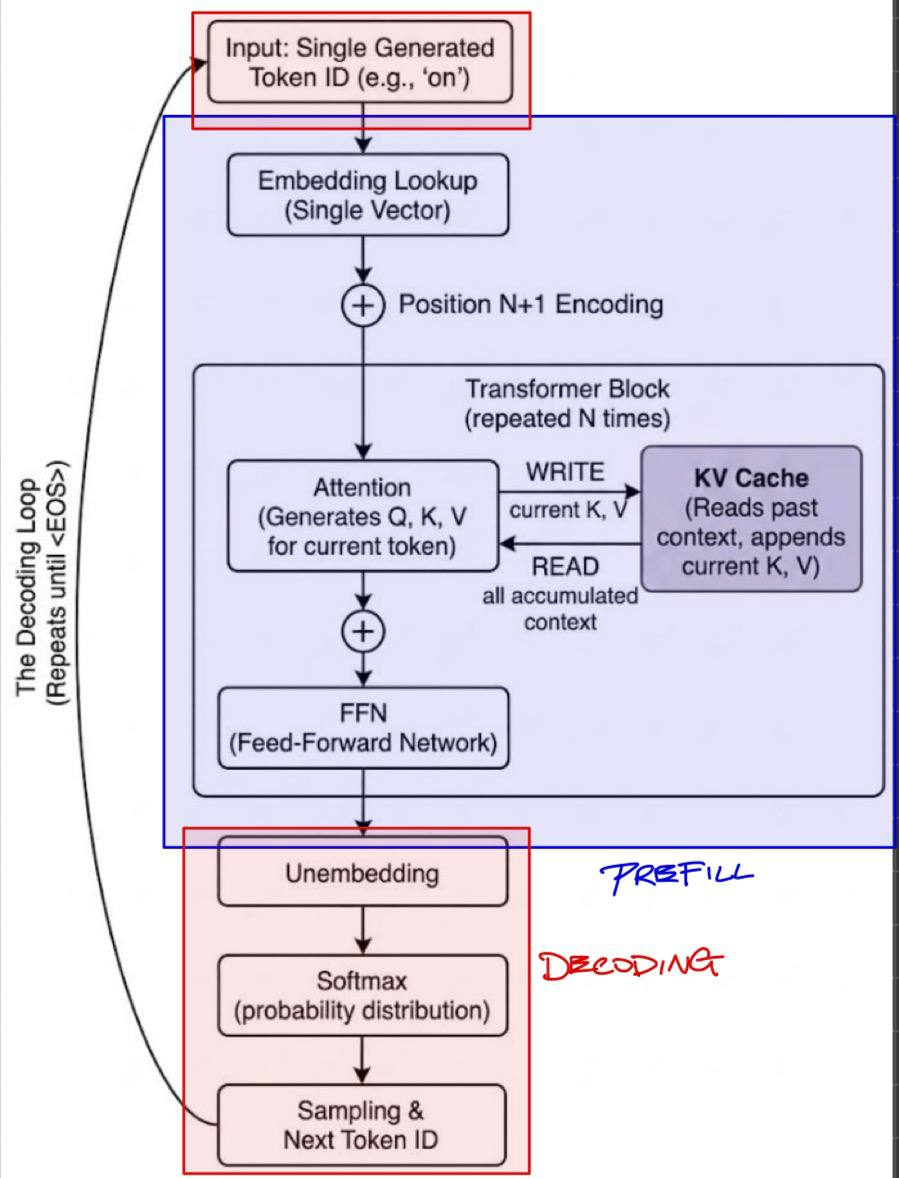
Now, if the word Mat is chosen, it is fed into the model as the next input token.

The model does the same thing again: computes Q, K, and V, performs attention, etc. The new K and V vectors are then appended to the KV cache for future generated tokens, while the new Query is answered by the K and V vectors that were previously cached.

This process repeats until a max token length is reached, or until the probabilistic outcome is to end the statement.